
What is a bell curve?
A bell curve, frequently referred to as the normal distribution, is a common form of a variable distribution. The word "bell curve" refers to the graph used to show a normal distribution, a uniform bell-shaped curve.
The peak on the curve, or the highest point of the bell, symbolizes the most likely event in a series of data (in this example, its mean, mode, and median). In contrast, all other potential events are uniformly dispersed around the mean, resulting in a curve that descends on either side of the peak. The standard deviation describes the breadth of the bell curve.
The concept of a bell curve
The word "bell curve" refers to a graphical representation of a normal probability distribution whose fundamental standard deviations from the mean produce the curved bell form. A standard deviation is an assessment that quantifies the variation of data dispersion in a range of variables around the mean. Conversely, the mean translates to the average of each data point in the data sequence or series and will be located at the peak of the bell curve.
Financial traders and economists often employ a normal probability distribution when examining the earnings of securities or the overall market stability. The fluctuation in finance refers to standard deviations that indicate an asset's profits. For instance, securities with a bell curve are often blue-chip stocks with fewer fluctuations and more consistent trend patterns. Traders estimate the predicted future earnings based on the normal probability distribution of an asset's previous performance.
A bell curve is frequently employed in statistics, where it may be broadly used, in addition to instructors who utilize it while comparing exam results. Bell curves are frequently used in performance management to place individuals who execute their jobs well in the normal distribution of the graph. The falling slope reflects the high and low achievers on each side. It might benefit bigger organizations when conducting performance evaluations or making management choices.
The features of a bell curve
The bell curve has complete symmetry. It converges towards the summit and gradually declines on each side. The highest point of a bell curve reflects the most likely occurrence in the data set, while the remaining events are evenly dispersed around the highest point. The more a value deviates from the mean, the less probable it will occur. Asymptotic ends near but never quite touch the horizontal plane (the x-axis).
The curve's apex correlates to the dataset's mean (recall that under a normal probability distribution, the mean simultaneously represents the median and the mode). A normal distribution's mode, median, and mean will all have similar values, depicted graphically by the curve's apex.
The normal distribution is called the bell curve since the probability distribution graph resembles a bell. The standard deviation measures the distribution of the data on the bell curve. The bell curve and standard deviation probability have many relevant links, including:
· Approximately 68% of the data is within one standard deviation.
· Approximately 95% of the data falls within two standard deviations.
· Approximately 99.7% of the data falls within three standard deviations.
The correlations mentioned above are called the 68-95-99.7 rule or the empirical rule. The empirical rule is often used to get the confidence interval for a normal distribution of probabilities.
Because of the broad uses of the normal probability distribution, the idea is immensely significant in statistics. The normal probability distribution, for example, describes the placement of random variables whose true distribution is uncertain.
The formula of the bell curve
Below is the equation for the bell curve:
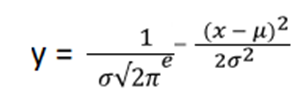
Where: μ = mean, σ = standard deviation, π = 3.14159, e = 2.71828.
· The mean, expressed as μ, represents the distribution's centre or middle.
· Because there is a square in the exponent, the horizontal symmetry around the vertical line is x = μ.
· The standard deviation is denoted by σ and is linked to the distribution's dispersion. The normal distribution will propagate out further as σ rises. The apex of the distribution is lower, and the tail of the distribution is greater.
· π represents a fixed pi and has a non-repeating decimal expansion.
· E, like pi, signifies an additional constant that is both transcendental and irrational.
· The coefficient has a negative sign, while the remaining elements are squared. As a result, the coefficient is always negative. As a result, the function grows for every x is less than the mean. When all x is greater than the mean, the reverse is true.
· A different approach of horizontal asymptote is the horizontal line y which equates to 0, which means that the function graph will not interact with the x-axis and will have a zero value.
· In Excel, the square root will adjust the formula, which indicates that when one integrates the function for seeking the area under the curve where the whole area would be under the curve, it is one, equivalent to 100%.
· This approach is similar to a normal distribution used to calculate probabilities.
Illustration of a bell curve
Standard deviation, measured as the dispersion of data in a sample around the mean, establishes the breadth of a bell curve. According to the empirical rule, 68 per cent of test results should lie within one standard deviation of the mean if 100 scores are gathered and used to create a normal probability distribution. The test was successfully administered if 95 out of 100 results were within two standard deviations of the mean. The following diagram shows that 99.7 per cent of the data points fall within three standard deviations of the mean. Long-tail data points beyond the three standard deviation range include exceptional outliers test scores such as 100 or 0.
The general importance of a bell curve
1. Natural phenomena and psychology exhibit bell-shaped distributions. Most continuous data in nature and psychology have a bell-shaped curve when assembled and plotted, making the normal distribution the major statistical probability distribution. Many continuous parameters, including intelligence level, body mass index, and blood pressure, are expected to follow a normal distribution frequency curve if we randomly select 100 people.
2. The data points in a sample must conform to a normal distribution for a parametric analysis of significance to be valid. For psychologists to utilize the most effective (parametric) statistical tests, data must follow a normal distribution. Non-parametric statistics is a less robust statistical test that may be used if the data does not fit a bell curve.
3. The equation for calculating z-scores from normal distribution's raw data. By transforming raw scores into z-scores, we may make data from a normal distribution more comparable. Using this method, scientists may compute the empirical rule or the percentage of observations within a certain deviation from the mean.
Interpretation and application of a bell curve
This function will be used to define the physical occurrences, the number of which is quite large. If there are many observations, it may be impossible to anticipate the item's result, but it will be possible to predict the aggregate behaviour of the data. Take the case of a gas jar maintained at a uniform temperature as an illustration. The probability of a single particle traveling at a given speed may be calculated using the normal distribution or bell curve.
When assessing the entire market's susceptibility or stock, the financial analyst employs the normal probability distribution, the bell curve. For instance, blue-chip stocks (those with a bell curve) tend to be less volatile and more consistently behave predictably. Therefore, they extrapolate future returns from the stock's historical bell curve, also known as the normal probability distribution.
The drawbacks of the bell curve
When evaluating performance, a bell curve grade tends to lump individuals into three distinct categories: bad, average, and excellent. It would be unfair to people in smaller groups if they were all forced to be placed in one of five categories so that the data would match a bell curve. They may all be ordinary at best, but since their ratings or grades must conform to a bell curve, some will inevitably be placed in the lowest tier. Data do not adhere to any ideal distribution. The distribution of values above and below the mean might sometimes be skewed. Fat tails (excess kurtosis) may also occur, increasing the likelihood of tail occurrences beyond what would be expected from a normal distribution.
Non-normal distributions vs the bell curve
The assumption of a normal probability distribution does not always hold in the corporate world. Non-normal distributions that do not match a bell curve are possible for the price of stocks and other assets.
The tails of a non-normal distribution are more extreme than a normal probability distribution, which looks like a bell curve. An increased likelihood of losses is signalled by a wider tail, discouraging investors.
Data distribution using the standard normal model
Plotting data on a graph is one method for determining how they are dispersed. Assuming the data is uniformly distributed, a bell curve may result. A bell curve has an insignificant proportion of points on both tails and a greater proportion on the curve's center. In the usual normal model, around 5% of the data provided will be in the "tails", while 90% will be in the middle. For instance, the normal distribution of a pupil's test results would reveal that 2.5 percent of students had extremely low scores and 2.5 percent received exceptionally high scores. The remainder will be in the center, neither too high nor too low.
The standard normal distribution may assist you in determining the areas you are doing well in and others you need to work harder on, owing to low score percentages. When you get more points in one subject than in another, you may believe you are superior in the subject with the higher score. However, this is frequently not the case.
You may only claim to be superior in a topic if your score is a specified number of standard deviations above the mean. The standard deviation indicates how closely your data is grouped around the mean; it enables you to compare various distributions with different sorts of data, even various means.
Contrasting the normal with the standard normal distribution
The mean and standard deviation are the two parameters that define a normal distribution. The standard normal distribution is a typical distribution with a standard deviation of 1 and a mean of zero. The normal distribution tables are built from this distribution.
The purpose of the bell curve in finance
When predicting probable outcomes important to investment, economists will often employ bell curves and other distributions of statistics. Based on the investigation, they might include future stock values, rates of future profits growth, possible rates of default, or other significant occurrences. Traders should carefully evaluate whether the outcomes under consideration have a normal distribution before using the bell curve in their study. Failure to do so may jeopardize the reliability of the final model.
Conclusion
Because of its similarity to a bell, the graph of a normal or the Gaussian distribution is occasionally known as the bell curve. This curve is a phenomenal statistical tool for calculating the probability of occurrences or outcomes for a true-valued random parameter. As a result, this method is occasionally used to generate financial investment forecasts. However, numerous factors of interest to financial firms have non-normal distributions, rendering applying the bell curve exceptionally risky.