
How Does the Empirical Rule Work?
The empirical rule is a commonly used method in data analysis to better understand the entire body under study.
Consider that for a given set of data, if the expected outcome will be normally distributed (i.e. 50 percent on either side), then the data will cluster around the mean or average. When graphed as a histogram, these measurements will form what’s commonly referred to as a bell curve.
Of course, not all of the measurements will align perfectly with the mean. Some may be close while others will be further away. This difference between the mean and the measurement is called variance. Mathematically, we can take the square root of the variance to calculate the standard deviation.
In statistics, the standard deviation is a useful metric because it can tell us how much of the data is close to the mean. This can be summarized using the empirical rule as follows:
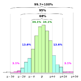
● 68.0 percent of the data lies within one standard deviation on either side of the mean
● 95.0 percent of the data lies within two standard deviations on either side of the mean
● 99.7 percent of the data lies within three standard deviations on either side of the mean
In other words, we can infer that based on the observed behavior of this sample we can reasonably predict that the majority of the population will fall within this three-sigma variation. For this reason, you may also sometimes hear the empirical rule referred to as the three-sigma rule or 68-95-99.7 rule.
How To Use the Empirical Rule
Suppose you work in a factory where bags are to be filled to 40 lbs each. Since 40 lbs is the target, you can reasonably expect a 50/50 chance that the bags will either be more or less than the target. Hence, since the data will be normally distributed, you can use the empirical rule as follows.
1) Collect the Measurements
As part of quality control, you weigh the last ten bags that were produced and record the following measurements:
39.8, 40.0, 40.3, 39.6, 40.1, 39.7, 40, 40.1, 39.9, 40.2
2) Find the Mean
Based on this data set, you calculate the mean, μ. This can be done by adding all of the measurements together and dividing them by the number of samples. Software such as Excel or Google Sheets can perform this calculation automatically.
For our example, the mean is found to be:
μ = 39.97
3) Find the Standard Deviation
For the same data set, you also calculate the standard deviation, σ. Standard deviation is found by calculating the variance of each measurement and then taking the square root. Again, this calculation can be simplified using Excel or Google Sheets.
For our example, the standard deviation is:
σ = 0.21
4) Emphiral Rule Conclusions
Using the empirical rule, we can say that for all the bags being filled:
● 68 percent of the product will weigh between 39.97 +/- (1 x 0.21) = 40.18 and 39.76 lbs
● 95 percent of the product will weigh between 39.97 +/- (2 x 0.21) = 40.39 and 39.55 lbs
● 99.7 percent of the product will weigh between 39.97 +/- (3 x 0.21) = 40.6 and 39.34 lbs
If quality control required that the product weighs +/- 1 lb, then we could say that this process was within tolerance.
However, if the requirement was tighter and required a variation of less than +/- 0.5 lbs, then we could say that the process does not meet the requirements. Hence, some adjustments may need to be done to fill the bags more accurately.
What Industries Use the Empirical Rule?
In the previous example, manufacturing is just one of the many places where the empirical rule can be used. In reality, it can be applied across dozens of industries wherever statistical methods assist in data analysis. A few other examples include:
● Science - Drawing conclusions after testing a hypothesis and analyzing the data.
● Business and marketing - Increasing sales by researching the demographics of customers and tailoring advertising messages to better reach the intended audience.
● Finance and Accounting - Using past results to draw conclusions about how the business or investment may perform going forward.
● Sports - Performance characteristics of certain players or teams overall.
● Technology - How quickly or accurately software can perform a routine.
● Health care - Applications such as pharmaceutical development, treatment effectiveness, or the risk of transmitting an illness.
● Etc.
Empirical Rule vs Chebyshev’s Theorem
While the empirical rule can be used to forecast trends about data sets with a normal distribution, these same generalizations cannot be made when the data is not normally distributed. In this case, we must apply an alternate set of guidelines known as Chebyshev’s Theorem.
Here are the conclusions that can be drawn when we use Chebyshev’s Theorem:
● 3/4 of the data will be within two standard deviations from the mean
● 8/9 of the data will be within three standard deviations from the mean
● For any whole number k greater than one, 1 – 1/(k^2) of the data will like within k standard deviations from the mean
The Bottom Line
The empirical rule can be used across a wide variety of industries to analyze data and forecast trends. Knowing ahead of time that at least 99.7 percent of the measurements will fall within three standard deviations, professionals can make educated guesses about the population as a whole.
The empirical rule works when data is normally distributed in the form of a bell curve. In situations where it is not, an alternate concept known as Chebyshev’s Theorem should be applied.